Training output
The train_seqstructhmm script writes all its output into the given output directory (by default: the current directory, configurable with the --output_directory parameter). There, it creates a job directory with the name <job_name>_<date>_<time>. During the runtime of the script, the following files are written:
Logs:
<job_name>_verbose.log<job_name>_numbers.log
Model graphs:
graphs/graph_<iteration>.pngfinal_graph.png
Model files:
models/model_<iteration>.xmlfinal_model.xml
Sequence logos:
logo_global.pnglogo_global.txtlogo_hairpin.pnglogo_hairpin.txtlogo_best_sequences.pnglogo_best_sequences.txt
Logs
The verbose log <job_name>_verbose.log is identical to the standard output of the script. Each line contains the current time and the logging level. At the top, the full command that called the script and the chosen options are printed. In every training iteration, the log contains the current loglikelihoods of the input data given the model and the current information content of the model in six different variants. The information content is either obtained from the top-scoring 1000 sequences or computed directly from the model. Additionally, we distinguish sequence, structure, and sequence-structure information content. At the end, the log contains the number of training iterations and the locations of the final model graph and model file.
The numbers log <job_name>_numbers.log contains the same information for each iteration as the verbose log but in a condensed, comma-separated format. Each line holds information for one iteration. The columns are:
- Iteration number
- Sequence loglikelihood
- Sequence-structure loglikelihood
- Average per-position information content of sequence (from top 1000 sequences)
- Average per-position information content of structure (from top 1000 sequences)
- Average per-position information content of sequence and structure (from top 1000 sequences)
- Average per-position information content of sequence (from model)
- Average per-position information content of structure (from model)
- Average per-position information content of sequence and structure (from model)
Model graphs
The graph images provide a clear and intuitive visualization of the motif that has been found by training the model. HMMs are graphical models that lend themselves to a visualization as a graph. The states and emissions of an HMM can be depicted as nodes while the transition and emission probabilities can be represented as weighted edges between the nodes.
As an example, the following image shows the output of ssHMM after it has been trained on a CLIP-Seq dataset of the RBP DGCR8. The states of the ssHMM, including the start and the end state, are represented by rectangular boxes that are arranged into rows and columns. The columns represent the motif positions while the rows represent the five structural contexts of RNA.
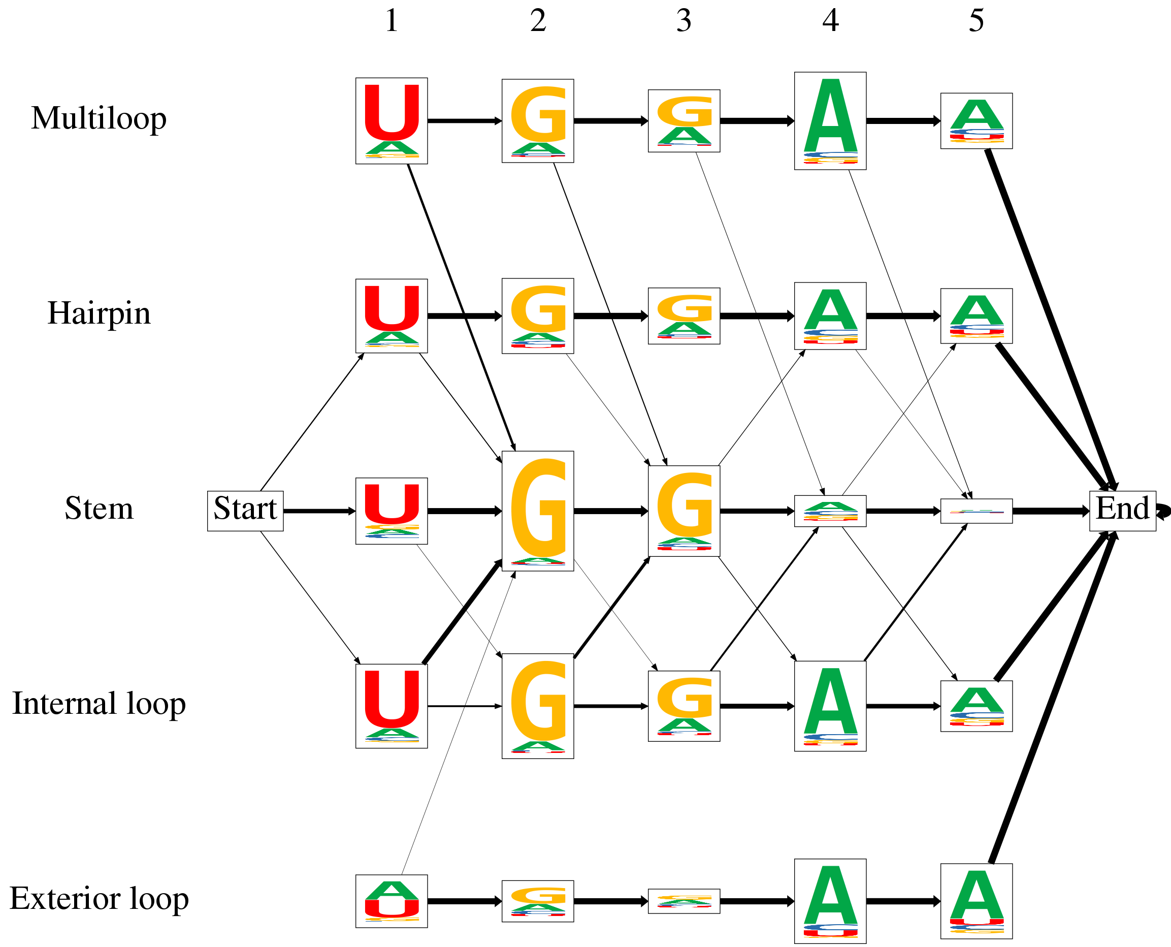
The emissions of the ssHMM are the four nucleotides A, C, G, and T. Sequence logos are used to visualize the emission probabilities of each state directly in the state’s box. The heights of the nucleotide letters in the sequence logos depend on two properties: Firstly, the relative height of a letter reflects its prevalence in this state, i.e. its emission probability. Secondly, the total height of the stack of four nucleotides is scaled according to the information content of the emission probabilities in this state. Consequently, states with a high information content stand out because of their size while those with more uniform emission probabilities are smaller. Different colors for the four nucleotides make it very easy to immediately grasp the sequence motif defined by the ssHMM. For this concrete RBP, the sequence motif is UGGAA.
The transition probabilities between the states are visualized as arrows. The thicker an arrow between two states, the more likely is a transition between the two. The most important transitions originate from the start state because they determine in which structural context the motif starts. Often, the motif remains in one particular context for its entire length (as can be seen for the hairpin and stem context in the graph above} but not for the internal loop context). To reduce clutter and increase clarity, unlikely transitions with a probability of less than 0.05 are completely omitted. This can be observed, for example, between the start state and both multiloop and exterior loop contexts. The RBP depicted in the graph above preferably binds stem regions of RNA but to a lesser extent also hairpin loops and internal loops.
By default, the training script outputs a graph image of the current state of the model every i iterations (as defined by the --termination_interval argument) into the graphs/ subdirectory. After the training is completed, the final model graph is written into the file final_graph.png.
Model files
Every i iterations, the model in its current state is exported as an XML file into models/model_<iteration>.xml. After the training is completed, the final model is exported as final_model.xml. The exported XML files hold all model parameters (e.g. states, emissions, transition probabilities, emission probabilities and initial probabilities). Advanced users can use the ghmm Python package to import and use the exported HMMs further.
Sequence logos
Beside the comprehensive visualization of the model as a model graph, ssHMM supports the visualization of the trained motif as simple sequence logos. Three different sequence logos are produced after completion of the training:
- a global sequence logo
logo_global.pngwhich shows the average sequence motif over all structural contexts - a hairpin sequence logo
logo_hairpin.pngwhich shows the sequence motif in the hairpin context - a sequence logo
logo_best_sequences.txtwhich is generated from the 1000 sequences that are most likely under the model
All three sequence logos are exported as PNG image and text file. The text files have the following format: The first line lists the emissions (in most cases, A, C, G and T). Each subsequent line contains one motif position with the tab-separated probabilities of the respective emissions.